3 Logistic Regression
3.1 Logistic Regression
Now that we understand simple linear regression, we can move to a slightly different type of model called logistic regression.
Logistic regression is used when the dependent variable (y) is categorical, most often binary (e.g., 0 or 1, yes or no, true or false).
Instead of predicting a continuous value, logistic regression predicts a probability.
In other words, it helps answer:
What is the probability that an outcome belongs to a certain category?
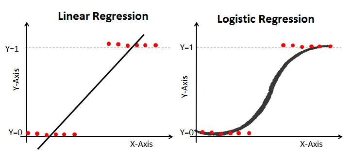
Example of linear vs logistic regression from (https://www.analyticsvidhya.com/blog/2021/08/conceptual-understanding-of-logistic-regression-for-data-science-beginners/)
3.2 Logic
Imagine you are trying to predict whether a student passes an exam based on how many hours they studied.
- Output is not a number
- Output is a category: pass (1) or fail (0)
Instead of drawing a straight line, logistic regression fits an S-shaped curve that keeps predictions between 0 and 1.
3.3 Equation
Logistic regression models the log-odds of the outcome:
\[ \log\left(\frac{p}{1 - p}\right) = a + bx \]
where:
- p = probability of outcome = 1
- log (p/1-p) = log-odds (also called the logit)
- a = intercept
- b = coefficient
- x = independent variable
3.4 From Log-Odds to Probability
The log-odds can be converted back into a probability using the logistic (sigmoid) function:
\[ p(x) = \frac{1}{1 + e^{-(a + bx)}} \]
3.5 Example
Let’s create a simple dataset:
import numpy as np
import pandas as pd

df = pd.DataFrame({
    "hours": [1, 2, 3, 4, 5, 6],
    "pass":  [0, 0, 0, 1, 1, 1]
})

df
3.6 Visualizing the Data
import matplotlib.pyplot as plt

plt.scatter(df["hours"], df["pass"])
plt.xlabel("Study Hours")
plt.ylabel("Pass (0 = No, 1 = Yes)")
plt.title("Study Hours vs Passing")
plt.show()
3.7 Fitting a Logistic Regression Model
from sklearn.linear_model import LogisticRegression

X = df["hours"].values.reshape(-1, 1)
y = df["pass"].values

model = LogisticRegression()
model.fit(X, y)

intercept = model.intercept_[0]
coefficient = model.coef_[0][0]

print("Intercept (a):", intercept)
print("Coefficient (b):", coefficient)
3.8 Predicting Probabilities
probabilities = model.predict_proba(X)[:, 1]

df["probability"] = probabilities
df
3.9 Making Predictions
predictions = model.predict(X)

df["prediction"] = predictions
df
3.10 Visualizing the Logistic Curve
x_range = np.linspace(df["hours"].min(), df["hours"].max(), 100).reshape(-1, 1)
y_prob = model.predict_proba(x_range)[:, 1]

plt.scatter(df["hours"], df["pass"], label="Observed data")
plt.plot(x_range, y_prob, color="red", label="Logistic curve")
plt.xlabel("Study Hours")
plt.ylabel("Probability of Passing")
plt.legend()
plt.show()
3.11 What does the coefficient mean?
The coefficient (b) tells us how (x) affects the log-odds of the outcome:
- If (b > 0): increasing (x) increases the log-odds (and probability) of outcome = 1
- If (b < 0): increasing (x) decreases the log-odds (and probability)
- If (b = 0): no relationship
3.12 Residuals
In logistic regression, residuals are interpreted differently than in linear regression.
- We compare observed values (0 or 1) with predicted probabilities
3.13 Why Logistic Regression?
- Keeps predictions between 0 and 1
- Works well for classification problems
- Easy to interpret
3.14 Key Assumptions of Logistic Regression
- Independent observations
- Linear relationship between predictors and log-odds
- No strong multicollinearity
- Large sample size
3.15 Summary
- Logistic regression is used for classification
- It models log-odds using a linear equation
- Probabilities are obtained using the logistic function
- Outputs can be converted into categories
- Coefficients show how predictors affect the likelihood of an outcome