6 Spatial Autocorrelation
6.1 Spatial Autocorrelation
In spatial data, values are often not independent of location.
Instead, nearby places tend to influence each other.
This is called spatial autocorrelation.
In simple terms, do nearby locations tend to have similar values, or different values?
6.2 Positive vs Negative Spatial Autocorrelation
Spatial autocorrelation can take a few main forms:
- Positive
- Negative
- Random
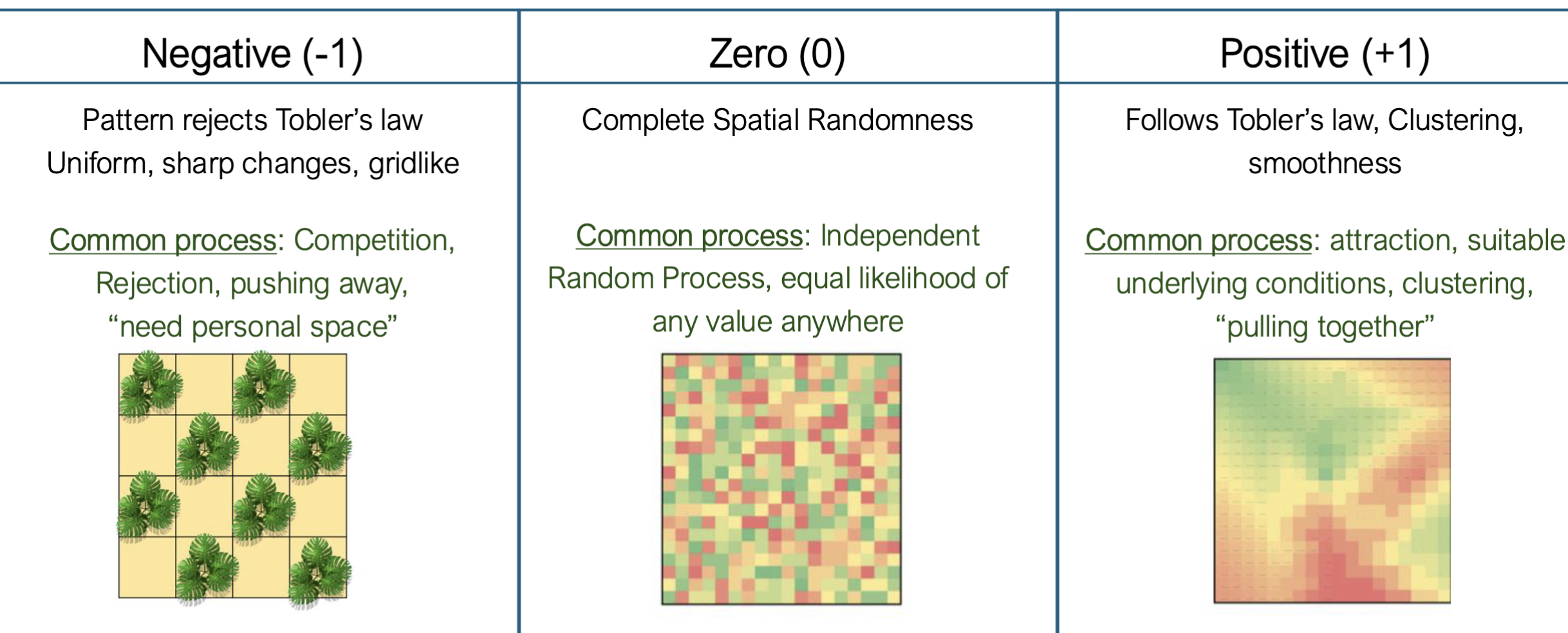 Example of Autocorrelation types from PSU Geog560 Lecture by Helen Greatrex.
6.3 Positive Spatial Autocorrelation
Positive spatial autocorrelation means similar values cluster together in space
6.3.1 What it looks like:
- High values near high values
- Low values near low values
- Smooth, clustered patterns
6.3.2 Key idea:
“Like values attract like values in space”
6.4 Negative Spatial Autocorrelation
Negative spatial autocorrelation means nearby values tend to be very different from each other
6.4.1 What it looks like:
- High values next to low values
- Checkerboard or alternating patterns
- Strong spatial contrast
6.4.2 Key idea:
“Opposites are next to each other in space”
6.5 No Spatial Autocorrelation
Sometimes there is:
- no clear spatial pattern
- values appear randomly distributed
This means that location does not help explain the value
6.6 Why This Matters
Understanding spatial autocorrelation is important because:
- many statistical methods assume independence
- spatial data often violates this assumption
- ignoring spatial structure can lead to incorrect conclusions
6.7 Moran’s I
A common way to measure spatial autocorrelation is Moran’s I.
It tells us whether spatial patterns are clustered, random, or dispersed in one global statistic.
6.8 Moran’s I Formula
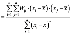
where:
- n = number of spatial units
- xi, xj = value at location i, j
- x bar = mean value
- Wij = spatial weight between locations i and j (from Spatial Weight Matrix)
6.9 Interpreting Moran’s I
- I > 0 → positive spatial autocorrelation (clustering)
- I ≈ 0 → no spatial structure (random pattern)
- I < 0 → negative spatial autocorrelation (dispersion)
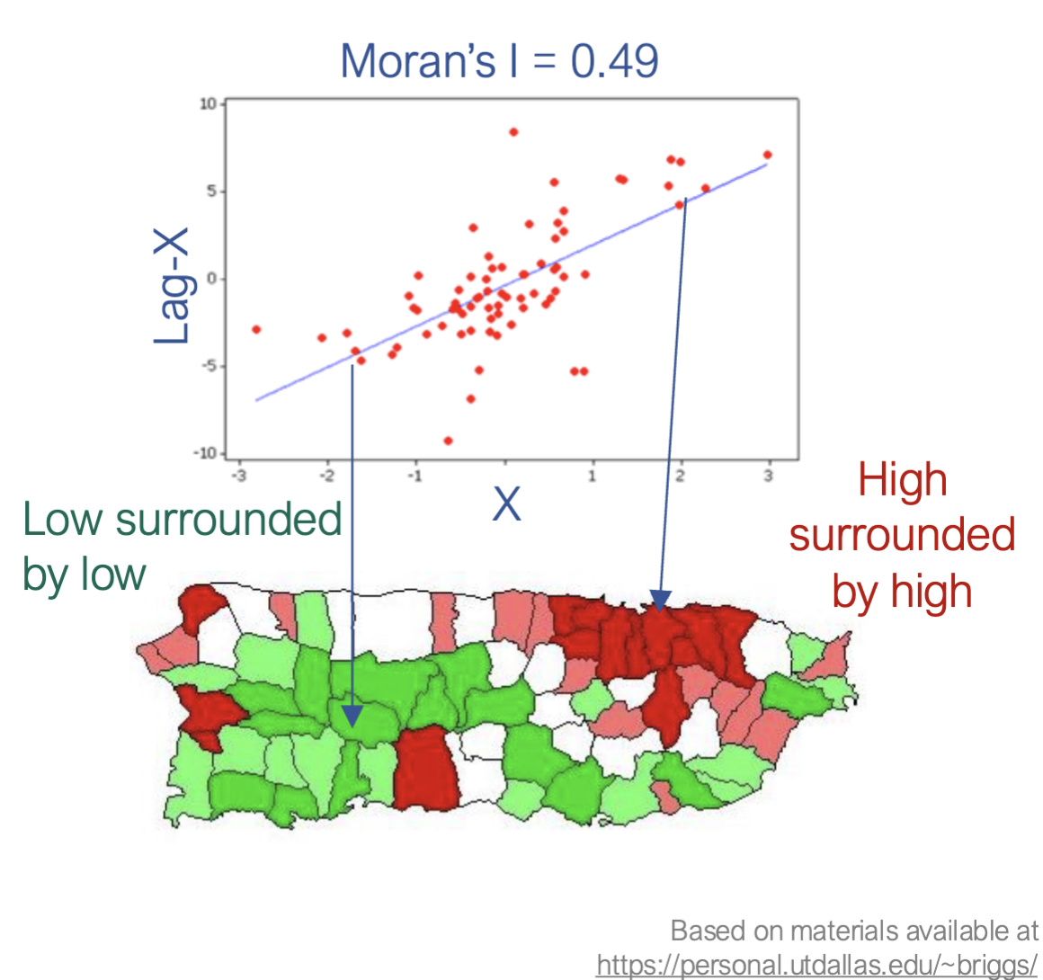 Example of Moran’s I from PSU Geog560 Lecture by Helen Greatrex. Based on materials available at https://personal.utdallas.edu/~briggs/
6.10 Connection to Spatial Weights
Moran’s I depends on the spatial weight matrix:
- rook neighbors → stricter definition of adjacency
- queen neighbors → broader definition of adjacency
So changing how we define “neighbors” can change the result.
6.11 Why This Is Important
Spatial autocorrelation tells us that:
- space is structured, not random
- nearby observations carry information about each other
- spatial relationships must be explicitly accounted for in analysis
6.12 Local Spatial Autocorrelation (LISA)
While Moran’s I measures spatial autocorrelation across an entire study area, it does not show where clustering occurs and only provides one global statistic of autocorrelation.
To identify local spatial patterns, we use:
LISA — Local Indicators of Spatial Association
LISA measures how each location relates to its neighbors.
In simple terms, is this location surrounded by similar values, or different values?
6.13 What LISA Identifies
LISA helps detect four main spatial patterns:
- High–High (HH) → high values surrounded by high values
- Low–Low (LL) → low values surrounded by low values
- High–Low (HL) → high value surrounded by low values
- Low–High (LH) → low value surrounded by high values
6.14 Cluster vs Outlier
6.14.1 Spatial Clusters
These indicate areas where nearby values are similar:
- High–High → hotspot / cluster of high values
- Low–Low → coldspot / cluster of low values
These are examples of positive local spatial autocorrelation.
6.14.2 Spatial Outliers
These indicate locations that differ from their neighbors:
- High–Low → unusually high value in a low-value neighborhood
- Low–High → unusually low value in a high-value neighborhood
These are examples of negative local spatial autocorrelation.
6.15 Interpreting a LISA Map
A LISA cluster map often uses colors to show patterns:
- High–High → hotspot
- Low–Low → coldspot
- High–Low → high outlier
- Low–High → low outlier
- Not significant → no meaningful local spatial pattern detected
This helps identify where spatial clustering is strongest.
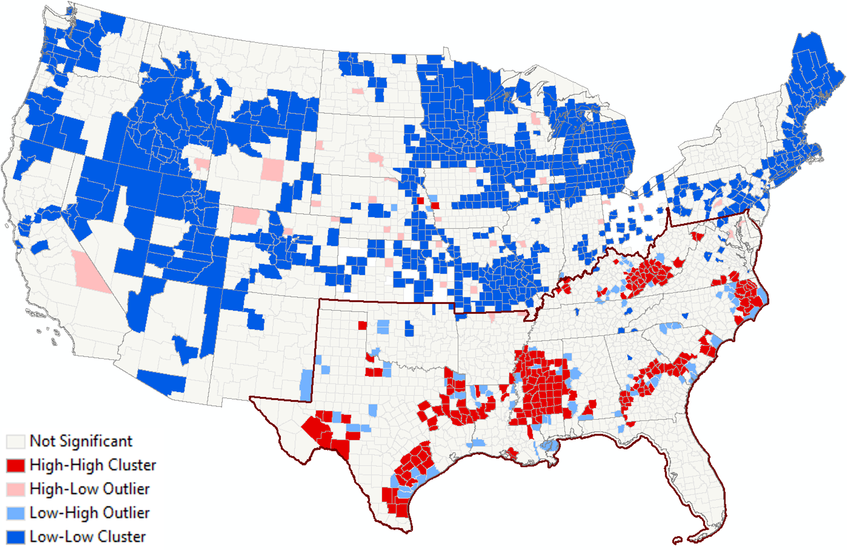 Example of LISA Map. Kim, Ayoung & Green, John & Johnson-Gaither, Cassandra & Dobbs, G. Rebecca. (2026). Analyzing heirs’ property prevalence and spillover effects in the U.S. using spatial econometric analysis. Agricultural and Resource Economics Review. 54. 1-21. 10.1017/age.2025.10016 —
6.16 Relationship to Moran’s I
- Moran’s I = global pattern
- LISA = local pattern
Moran’s I answers: Is there spatial autocorrelation overall?
LISA answers: Where is spatial autocorrelation occurring?
6.17 Why LISA Matters
LISA is useful because it can reveal:
- hotspots
- coldspots
- spatial boundaries
- unusual outliers
- neighborhoods that behave differently from surrounding areas
6.18 Summary
- Spatial autocorrelation measures how values relate across space
- Positive autocorrelation = clustering of similar values; Negative autocorrelation = neighboring contrasts
- Moran’s I measures global spatial autocorrelation
- LISA measures local spatial autocorrelation
- LISA identifies clusters and outliers
- LISA helps show where spatial patterns occur