2 Simple Linear Regression (SLR)
2.1 Simple Linear Regression
Before diving into spatial regression, it is important to understand what regression is. The simplest regression model is called simple linear regression (SLR).
Simple linear regression is a statistical method that models the relationship between an independent variable (x) and a dependent variable (y) by fitting a straight line (line of best fit) to observed data.
In other words, SLR helps answer the question:
How does y change as x changes?
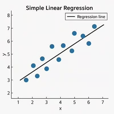
Example of linear regression from (https://sixsigmadsi.com/glossary/simple-linear-regression/)
2.2 Logic
Imagine you are trying to predict the cost of a house based on its size (square footage). If more square footage generally leads to higher housing costs, we can represent that relationship with a straight line.
SLR finds the line that best represents this trend in the data.
2.3 SLR Formula
The equation for a simple linear regression model is:
\[ y = a + bx + \varepsilon \] where:
- y = dependent variable (response)
- x = independent variable (predictor)
- a = intercept (value of (y) when (x = 0))
- b = slope (change in (y) per unit change in (x))
- epsilon = error term (difference between observed and predicted values)
2.4 What does the slope mean?
The slope (b) tells us how strongly (x) influences (y):
- If (b > 0): positive relationship
- If (b < 0): negative relationship
- If (b = 0): no relationship
2.5 Example
Let’s create a simple dataset:
import numpy as np
import pandas as pd

df = pd.DataFrame({
    "x": [1, 2, 3, 4, 5],
    "y": [2, 4, 5, 4, 5]
})

df
2.5.1 Visualizing the Data
Before fitting a regression model, it is important to visualize the relationship between variables.
Let’s create a simple dataset:
import matplotlib.pyplot as plt

plt.scatter(df["x"], df["y"])
plt.xlabel("x")
plt.ylabel("y")
plt.title("Scatter plot of x vs y")
plt.show()
2.5.2 Fitting a Simple Linear Regression Model
We can use scikit-learn to fit a regression model.
from sklearn.linear_model import LinearRegression

X = df["x"].values.reshape(-1, 1)
y = df["y"].values

model = LinearRegression()
model.fit(X, y)

intercept = model.intercept_
slope = model.coef_[0]

print("Intercept (a):", intercept)
print("Slope (b):", slope)
2.5.3 Plotting the Regression Line
y_pred = model.predict(X)

plt.scatter(df["x"], df["y"], label="Observed data")
plt.plot(df["x"], y_pred, color="red", label="Regression line")
plt.xlabel("x")
plt.ylabel("y")
plt.legend()
plt.show()
2.5.4 Residuals
\[ residual = y_{observed} - y_{predicted} \]
df["y_pred"] = y_pred
df["residuals"] = df["y"] - df["y_pred"]

df
2.5.5 Visualizing Residuals
plt.scatter(df["x"], df["residuals"])
plt.axhline(0)
plt.xlabel("x")
plt.ylabel("Residuals")
plt.title("Residual Plot")
plt.show()
2.5.6 Why Residuals Matter
- Large residuals indicate poor predictions
- Patterns in residuals suggest the relationship may not be linear
- A good model will have residuals randomly scattered around zero
2.6 Key Assumptions of SLR
- Linearity
- Independence of errors
- Constant variance of errors (homoscedasticity)
- Normally distributed errors
2.7 Summary
- SLR models the relationship between one predictor and one response
- It fits a straight line using (y = a + bx)
- Residuals help evaluate model performance